install the packages

# install.packages("pacman")
pacman::p_load(tidyverse, tidytext, rtweet) 

library(tidyverse) 
library(ggplot2)
library(tidytext)
library(rtweet)
library(knitr)

let’s go get some tweets

In recognition of today being ‘MayThe4th’ we will search for tweets using the #StarWars hash-tag.

starwars <- search_tweets(q = "#StarWars", n = 18000, include_rts = FALSE, `-filter` = "replies", lang = "en")

take a closer look

Check the first 10 tweets and then export them all as a CSV file.

starwars %>%
  head(10) %>%
  select(created_at, screen_name, text, favorite_count, retweet_count)

## # A tibble: 10 x 5
##    created_at          screen_name  text            favorite_count retweet_count
##    <dttm>              <chr>        <chr>                    <int>         <int>
##  1 2020-06-11 06:56:36 selvadt      "#starwars\nEp…              0             0
##  2 2020-06-11 06:55:36 GalaxieStar… "#StarWars #Th…              0             0
##  3 2020-06-05 15:08:23 GalaxieStar… "#Disney - Les…             16             1
##  4 2020-06-11 06:54:39 massiveboy90 "#StarWars, st…              0             0
##  5 2020-06-11 06:54:35 DigitalWhis… "He's on Endor…              0             0
##  6 2020-06-03 12:29:15 DigitalWhis… "THEY WERE FRA…              8             1
##  7 2020-06-10 11:43:47 DigitalWhis… "AWESOME!\n\nV…              6             2
##  8 2020-06-11 06:53:13 McBricksRev… "Hands up you …              0             0
##  9 2020-06-05 07:05:09 McBricksRev… "Affirmative. …              1             1
## 10 2020-06-09 06:44:00 McBricksRev… "I am able to …              1             1

Why don’t we save all these tweets as a CSV file.

write_as_csv(starwars, "starwars-tweets.csv")

let’s dig a bit deeper

Let’s look at the timeline of our tweets.

ts_plot(starwars, "hours") +
  labs(x = NULL, y = NULL,
       title = "Frequency of tweets with the #starwars hashtag",
       subtitle = paste0(format(min(starwars$created_at), "%d %B %Y"), " to ", format(max(starwars$created_at),"%d %B %Y")),
       caption = "Data collected from Twitter's REST API via rtweet") +
  ggplot2::theme_classic()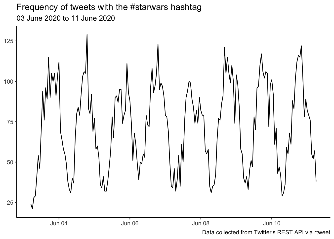

What was the top tweeting location.

starwars %>%
  filter(!is.na(place_full_name)) %>%
  count(place_full_name, sort = TRUE) %>%
  top_n(5)

## # A tibble: 5 x 2
##   place_full_name             n
##   <chr>                   <int>
## 1 Mississippi, USA           26
## 2 San Francisco, CA          26
## 3 Louisville, KY             19
## 4 Sydney, New South Wales    14
## 5 Florida, USA               12

The most retweeted tweet.

starwars %>%
  arrange(-retweet_count) %>%
  slice(1) %>%
  select(created_at, screen_name, text, retweet_count)

## # A tibble: 1 x 4
##   created_at          screen_name   text                           retweet_count
##   <dttm>              <chr>         <chr>                                  <int>
## 1 2020-06-05 23:06:00 MissStreetli… "Finally finished this drawin…          1177

The most liked tweet.

starwars %>%
  arrange(-favorite_count) %>%
  top_n(5, favorite_count) %>%
  select(created_at, screen_name, text, favorite_count)

## # A tibble: 5 x 4
##   created_at          screen_name   text                          favorite_count
##   <dttm>              <chr>         <chr>                                  <int>
## 1 2020-06-05 18:26:30 HamillHimself "THANK YOU to #HealthCareHer…           5674
## 2 2020-06-05 23:06:00 MissStreetli… "Finally finished this drawi…           5042
## 3 2020-06-10 12:04:09 Savannahbard… "I N S T I N C T\n__________…           4080
## 4 2020-06-05 13:50:59 jimmykimmel   "Our #HealthCareHero of the …           3569
## 5 2020-06-09 02:11:33 TheSWU        "What if feels like to be a …           3474

Who were the top tweeters.

starwars %>%
  count(screen_name, sort = TRUE) %>%
  top_n(10) %>%
  mutate(screen_name = paste0("@", screen_name))

## # A tibble: 10 x 2
##    screen_name          n
##    <chr>            <int>
##  1 @bpdstarwars       578
##  2 @tpnalliance       145
##  3 @ST4RW4RS          136
##  4 @rcmadiax          128
##  5 @StarWarsRP        123
##  6 @FanthaTracks       95
##  7 @VintageStarWars    92
##  8 @JediNewsNetwork    82
##  9 @MentorSkywalker    78
## 10 @CoolDealCA         70

What was the most used emoji.

# install.packages("devtools")
devtools::install_github("hadley/emo")

library(emo)
starwars %>%
  mutate(emoji = ji_extract_all(text)) %>%
  unnest(cols = c(emoji)) %>%
  count(emoji, sort = TRUE) %>%
  top_n(10)

## # A tibble: 10 x 2
##    emoji     n
##    <chr> <int>
##  1 🔗      623
##  2 😂      278
##  3 👉      158
##  4 💥      153
##  5 ❤️      137
##  6 😍      124
##  7 🤣      102
##  8 💚       86
##  9 😁       86
## 10 💙       78

What were the top 10 hashtags.

starwars %>%
  unnest_tokens(hashtag, text, "tweets", to_lower = FALSE) %>%
  filter(str_detect(hashtag, "^#"),
         hashtag != "#MayThe4th") %>%
  count(hashtag, sort = TRUE) %>%
  top_n(10)

## # A tibble: 10 x 2
##    hashtag               n
##    <chr>             <int>
##  1 #StarWars          9600
##  2 #starwars          4168
##  3 #eBay               633
##  4 #TheMandalorian     439
##  5 #LEGO               298
##  6 #Disney             261
##  7 #BlackLivesMatter   241
##  8 #babyyoda           232
##  9 #disney             222
## 10 #marvel             214

Top mentions.

starwars %>%
  unnest_tokens(mentions, text, "tweets", to_lower = FALSE) %>%
  filter(str_detect(mentions, "^@")) %>%  
  count(mentions, sort = TRUE) %>%
  top_n(10)

## # A tibble: 10 x 2
##    mentions           n
##    <chr>          <int>
##  1 @starwars        306
##  2 @HamillHimself   206
##  3 @JohnBoyega      188
##  4 @YouTube         161
##  5 @Disney           86
##  6 @ahmedbest        83
##  7 @davefiloni       80
##  8 @eBay             73
##  9 @Poshmarkapp      73
## 10 @disneyplus       61

a slice of text analysis

Let’s examine the most frequently used words in these tweets.

words <- starwars %>%
  mutate(text = str_remove_all(text, "&amp;|&lt;|&gt;"),
         text = str_remove_all(text, "\\s?(f|ht)(tp)(s?)(://)([^\\.]*)[\\.|/](\\S*)"),
         text = str_remove_all(text, "[^\x01-\x7F]")) %>%
  unnest_tokens(word, text, token = "tweets") %>%
  filter(!word %in% stop_words$word,
         !word %in% str_remove_all(stop_words$word, "'"),
         str_detect(word, "[a-z]"),
         !str_detect(word, "^#"),         
         !str_detect(word, "@\\S+")) %>%
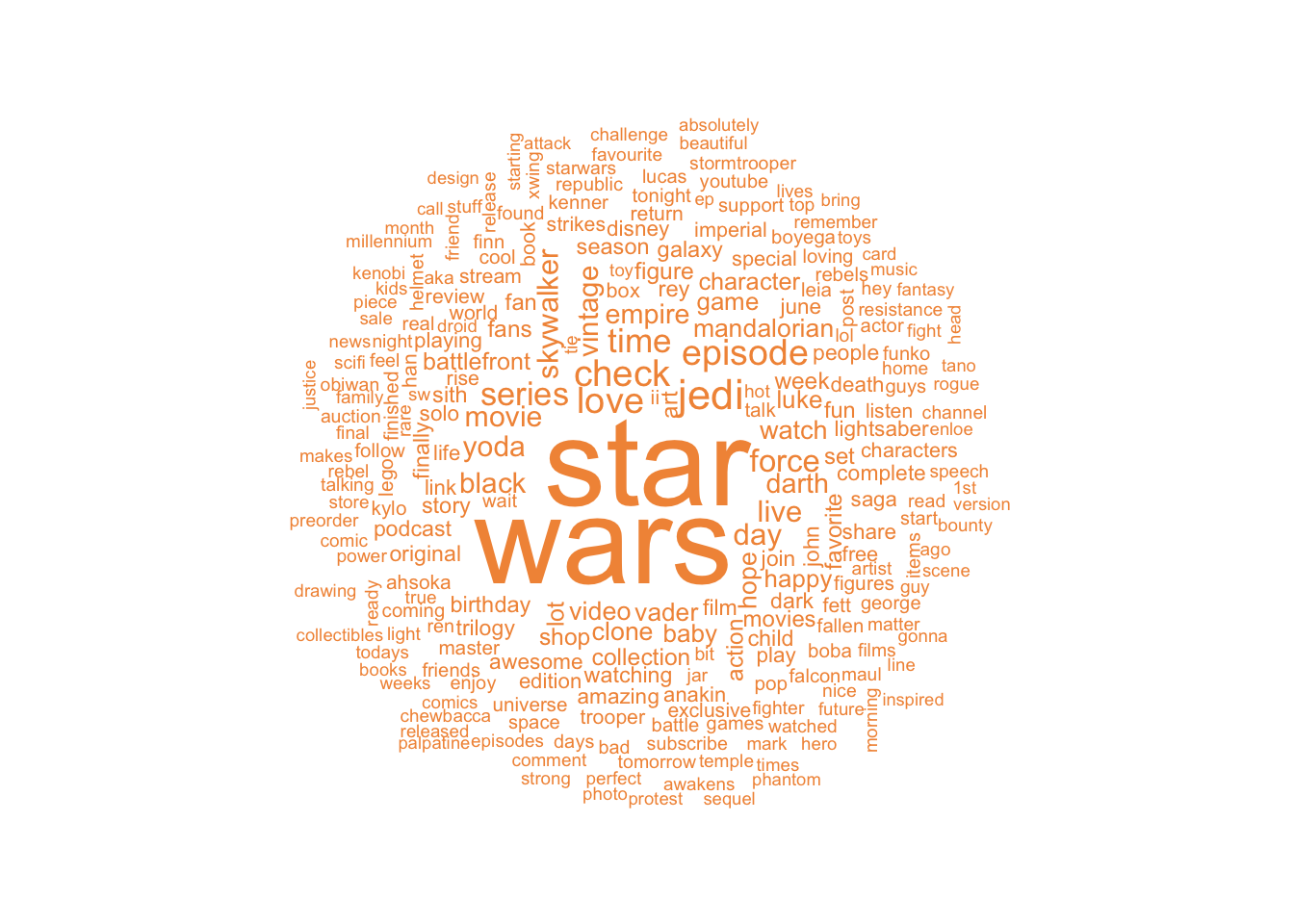
  count(word, sort = TRUE)

Finally - let’s use the wordcloud package to create a visualisation of the word frequencies.

library(wordcloud)
words %>%
  with(wordcloud(word, n, random.order = FALSE, max.words = 250, colors = "#F29545"))